

Discussions with many of our customers have revealed that when a laboratory compares two methods or instruments as part of their verification, they usually calculate the correlation coefficient. If we ask them, what conclusions can one make out of this value, they are rarely able to answer this question.
Are you relying on correlation coefficient in your verifications? If you are, you probably have a problem and you don’t even know it. But don’t worry, we have a solution for you.
But first, here’s why focusing into correlation coefficient in verifications is a bad practice and poor indicator of quality.
What does correlation coefficient mean?
Pearson correlation coefficient describes the strength of the linear relationship between two variables (variables being e.g. two methods for detecting the same analyte). If correlation r=1, a linear equation perfectly describes the relationship between the two. A value r=0 would imply that there’s no linear correlation. And r=-1 would point to inverse correlation, i.e. one variable decreases while the other one increases.
What does this mean in practice?
What good correlation reveals?
Imagine that we have e.g. one commercial and one in-house method that we are comparing. A correlation of r=1 would tell that the methods behave perfectly consistently as the concentration measured from the samples varies. Yet they do not necessarily give the same results.
In the image below you can see an example of two data sets that correlate with r=1. In the graph on the left, the x-axis of the graph represents the true concentration of our fictive test samples, and y-axis represents the concentrations measured from the samples. The dots on the graph are results measured from these samples. Orange dots represent results of Method 1 and blue dots represent results of Method 2.
The values given by these two methods for a sample are very different. Neither of them is linear throughout the whole concentration range. But since the shapes of these curves match, one giving results that are exactly three times the results of the other, they correlate perfectly.

Image 1: Example data with Pearson correlation coefficient r=1. On the left, results of both methods shown separately. In the middle, difference plot showing proportional Bland-Altman difference. On the right, regression plot showing results calculated using Passing-Bablok regression model.
The other graphs in the image are the difference plot (in the middle) and the regression plot (on the right) one would see when examining this kind of data in Validation Manager. They clearly show that there’s huge bias between these two methods.
So basically, what good correlation tells us is that we can make as good conclusions using Method 2 as we can using Method 1, but only if we know the bias between the two methods and are able to eliminate it from our results. Therefore bias is the information that you should be looking for when examining your comparison data.
How about poor correlation?
As we already noticed, identical shapes of the result sets give r=1, while differences between the shapes of the result sets cause correlation to be less than r=1. Now let’s look at two scenarios where correlation coefficient is not very good.
Poor precision causes poor correlation
One possible reason for poor correlation in a method verification is random error related to the results. But this is not information that we should be looking for when examining our comparison data.
For example in the image below you can see this kind of a data set, where bias is mostly small but there’s lots of variance in the results. In the upper left corner we again have results of both methods plotted separately. Below it you can find the difference plot. The lower right corner shows the regression plot. Upper right corner shows bias as function of comparative method results. We have set a bias goal for our data to make result interpretation easier. The green area in the graph represents concentrations where bias is acceptable (although the 95% CI lines suggest that we should measure more samples to be sure). The Pearson correlation coefficient for this data set is r = 0.886.
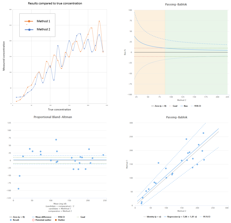
Image 2: Example data with Pearson correlation coefficient r=0.886, where main reason for poor correlation is problems with precision. In the upper left corner, results of both methods shown separately. In the lower left corner, difference plot showing proportional Bland-Altman difference. In the lower right corner, regression plot showing results calculated using Passing-Bablok regression model. In the upper right corner, bias plot showing behavior of relative bias as a function of comparative method results.
What can we deduce out of this kind of comparison data?
The problem is that when we are comparing two methods against each other, the results are affected by random error of both of these methods. When we look at the comparison data and the correlation coefficient obtained from the data, we have no means of finding out which method is to blame for the situation. That’s why a better way to gain knowledge of random error is to perform precision analysis for the method we are verifying. The point of a comparison is to measure the bias. As we can clearly see from the two examples above, correlation coefficient does not tell anything about the bias.
(There is though a protocol for evaluating bias and precision within the same study, but you cannot do that with this kind of a data set.)
Varying bias causes poor correlation
Another realistic reason for poor correlation is bias that varies over the measured concentration range. This may be related to systematic (but concentration dependant) problems in the verified method. But optionally it can be related to different behavior at some parts of the measurement range. For example, at the ends of the measurement range one method may give too big values while the other one gives too small values. In the middle, at clinically relevant levels, the methods may produce quite concordant results.
Below you can see an example of a data set like this. If the medically relevant concentrations are found in the area where bias is small, we can be happy with the results even though Pearson correlation coefficient for this data set is r= 0.877.
In this example we have set a stricter goal for the medically relevant concentration area. As you can see when looking at the bias plot, within that range bias goal is achieved (although the 95% CI lines suggest that we should measure more samples to be sure).
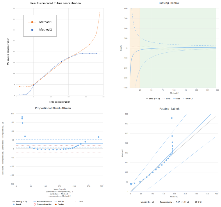
Image 3: Example data with Pearson correlation coefficient r=0.877, where main reason for poor correlation is bias varying as a function of concentration. In the upper left corner, results of both methods shown separately. In the lower left corner, difference plot showing proportional Bland-Altman difference. In the lower right corner, regression plot showing results calculated using Passing-Bablok regression model. In the upper right corner, bias plot showing behavior of relative bias as a function of comparative method results.
In this case, examining bias at relevant ranges or medical decision points gives more information about the method under verification than correlation coefficient gives.
So basically, poor correlation tells us that there may be a problem with the results. Yet it doesn’t tell us anything about the reason. To get knowledge about the reasons, you need to measure bias and precision. And if you set goals for your bias and precision, you will notice these problems even if you don’t pay attention to correlation.
So what does correlation coefficient tell about the data?
To revise, correlation coefficient describes the strength of the linear relationship between our two data sets. In method comparisons, the relevance of this information is not so clear. We are not really interested in knowing how close the shape of the result distribution from candidate method is to the one given by the comparative method. Instead we are interested in finding out whether the candidate method gives results that are good enough.
Every measurement has some intrinsic error. All methods have their own flaws. This causes effects similar to the exacerbated examples shown above.
The new method does not need to have weaknesses that are identical to the weaknesses of the old method. That’s why correlation does not answer our questions about whether the new method is good or not. It only gives us answers about the statistical properties of the data set obtained with these two methods. And as we saw already in the first example, good correlation does not guarantee absence of bias.
A more realistic example data set could look like in the image below. It’s real data from an actual verification, we’ve just masked the methods that were used. Now we don’t know the true concentrations so we don’t have the graph showing measured concentrations vs. true concentrations. Since it’s not evident that our data set would show either proportional or constant variation, we have two difference plots to visualize them both: proportional difference on the left and constant difference in the middle. Regression plot is on the right.
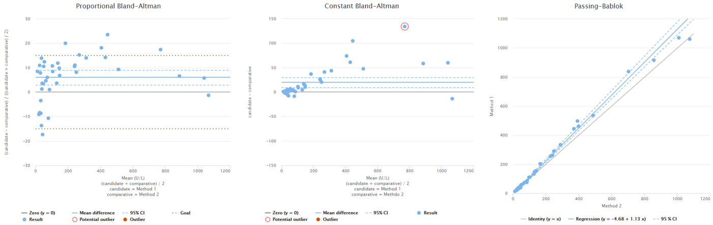
Image 4: Example data (from a real verification) with Pearson correlation coefficient r=0.996. On the left, difference plot showing proportional Bland-Altman difference. In the middle, difference plot showing constant Bland-Altman difference. On the right, regression plot showing results calculated using Passing-Bablok regression model.
Looking at these graphs it seems that there are areas of negative and positive bias and quite a lot of variance. The correlation coefficient of this data set is r = 0.996. Is that a good or a bad value for correlation? What does it tell about this data? (In case you are really wondering, the answer is nothing.)
What to look at instead of correlation?
Now we know that poor correlation doesn’t necessarily mean that there were relevant problems with the method under verification. And we have also seen that quite a good correlation doesn’t guarantee that there would not be problems with variation and varying bias. So there’s clearly no point in setting a goal for correlation coefficient as a measure of the quality of the method under verification.
Instead when examining our comparison data we should be interested in bias. We should find out how the bias changes as a function of concentration. That way we get understanding about the behavior of the test at different parts of the measuring range. We might even calculate bias values at specific concentrations where small differences in the results may change the medical conclusions one would make from the results. That’s basically what we should be doing: evaluating how big a bias is acceptable at different medical decision points or concentration ranges, and calculating whether our new method is within those limits.
To get better understanding about the behavior of the data above we have set range specific goals (constant goal for low concentrations, and smaller proportional goal for the medically most relevant concentration area – these are not real but invented for demonstration purposes). We have also set goals for two medical decision points. We can examine the behavior of bias using two graphs, one showing proportional bias (on the left in the image below) and one showing constant bias (on the right).

Image 5: Example data with Pearson correlation coefficient r=0.996. On the left, bias plot showing behavior of relative bias as a function of comparative method results. On the right, bias plot showing behavior of absolute bias as a function of comparative method results.
The method seems to be within our goals at low concentrations and concentrations above the medically relevant area (green background in the graph). Unfortunately a large part of the medically relevant area exceeds bias goals (orange area in the graph). The lower medical decision point (the green dot in the graph) is within goals, while the higher one (the red dot in the graph) is not. Had we set our goals differently, interpretation would be different. E.g. if we only had the lower medical decision point and the medically relevant area would be below 120 U/L, results would be ok.
If you are interested in knowing more about how to measure bias, here’s a brief introduction to bias calculations using Validation Manager. We will discuss bias in more detail in a later blog post.
On top of this analysis, we need to examine the precision in a separate study. For that we recommend using ANOVA protocol.
Why do so many still look at the correlation coefficient when doing method comparison?
If you are using ordinary linear regression model to calculate your bias, you need to do some statistical evaluations about your data to check whether the model is able to do a reliable bias estimation. One of these evaluations is checking correlation coefficient. It gives you some insight on whether your measuring range is wide enough to make the error related to your comparative method insignificant enough.
If you are doing your verification in Excel and need to do all the calculations there by yourself, it’s of course worth while to see if the statistical properties of the data set enable estimating bias with the simplest model available. So basically, if you are using OLR, correlation coefficient is one important indicator on whether your bias estimation can be trusted.
Unfortunately good correlation is not enough to guarantee that OLR gives good results. The model makes many other assumptions about the statistical properties of the data set that are rarely (if ever) encountered in medical measurement data. We will get back to this on a later blog post.
If you use Validation Manager, you don’t need to worry about the difficult calculations related to more complicated regression models. The results are calculated for you just as easily regardless of which model you use. Passing-Bablok (and in some cases linear or weighted Deming model) gives better results and saves you from monitoring your correlation coefficients.
If you’re still wondering about what else you should do in your verification process, be sure to check out our upcoming posts about this topic! We also offer statistical training to help laboratories make more precise conclusions about quality. You can contact us for more information here.
To be continued with
Accomplish more with less effort
See how Finbiosoft software services can transform the way your laboratory works.


