

In the end, what matters in a laboratory, is how reliable we can expect a single measured result to be. How do we estimate the effect that all possible error sources together can have on our measurements?
When verifying a test that gives quantitative results, we measure imprecision and bias. In many cases, these are done as separate studies. Imprecision is measured with repeated measurements of a small number of samples. In contrast, bias is typically measured using a rather large set of samples to cover the whole measuring range, and then calculating either average bias or bias as a function of concentration.
These are valuable techniques for verifications when we seek to understand the behavior and reliability of the method or instrument, possibly finding reasons for calibration or other adjustments.
But when we start to use the method for diagnostics, what truly matters is how close to the truth our results are overall. That’s a question where we don’t have a clear answer if we examine random error (i.e., imprecision) and systematic error (i.e., bias) separately. So how can we combine them to describe how close to the truth we can expect our results to be?
In this article, we introduce two approaches to this and discuss how they differ. We are talking about accuracy, meaning the closeness of agreement between a test result and the accepted reference value. Let’s start by looking at the components of accuracy: imprecision and bias and what they mean.
Standard deviation describes the variation in the data
Standard deviation (SD) and coefficient of variation (%CV) describe the variation in the data, i.e., observed random error either on an absolute scale (SD) or on a proportional scale (%CV). They give us the width of the distribution of the measured results if we measure the same sample again and again. If we took an infinite number of measurements, the distribution of the results should ideally look like Image 1. On the x-axis, we have the measured value (e.g., analyte concentration), and the dark blue curve shows the number of measurements given by each result. The vertical green line in the middle of the image shows the mean value of these results.

With about 68% probability, the measured result of our sample would be at most 1 SD away from the mean; in other words, they fall within the area with the darkest shade of blue in the distribution (between values Mean – SD and Mean + SD). With about 95% probability, the result is no more than 2 SD away from the mean, meaning that it’s found somewhere within the areas with darkest and second darkest shades of blue (between values Mean – 2 SD and Mean + 2 SD).
More generally, we can choose the confidence level we need, and present the corresponding maximum distance from the mean as Z * SD, where Z is a factor we can select based on our confidence level. Then we can say that for our purposes, the variation in the data is well enough described by saying that results tend to be between values Mean – Z * SD and Mean + Z * SD.
The bigger we choose Z to be, the smaller the proportion of results that will not meet this condition. In diagnostics, it’s common to choose 95% confidence, leading to Z = 2.
Bias tells us where the distribution is compared with true value.
In most cases, we also have systematic errors in our measurements. Systematic error is called bias, and it tells us how far the mean of the distribution is from the true value and which of the two is higher:
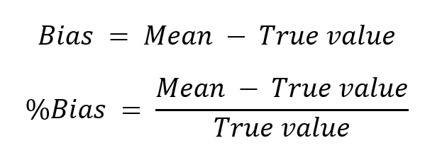
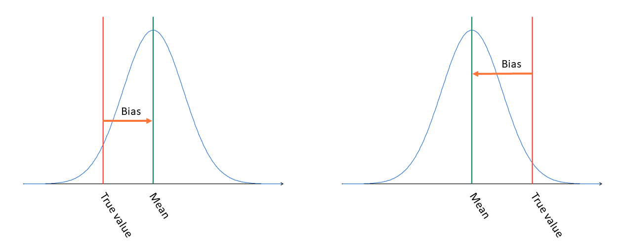
So, a positive bias means that our measured results tend to be somewhat higher than the true concentration in the sample (on the left in Image 2), and a negative bias means that the measured results tend to be lower than the true value (on the right in Image 2). As we can see in Image 2, a positive bias does not mean that every result would be larger than the true value; it’s just that, on average, they are larger. Bias and the width of the distribution together help us find an estimation for how accurate our measured results are overall.
Total analytical error
Total analytical error (TAE) represents the overall error that we find in a test result. It gives an upper limit on the total error of a measurement with a selected level of confidence. It was introduced in 1974 by Westgard, Carey and Wold (1). It is explained in more detail in a later AACC article by Westgard and Westgard (2). Also worth reading are CLSI EP29 (4) and EP21 (5).
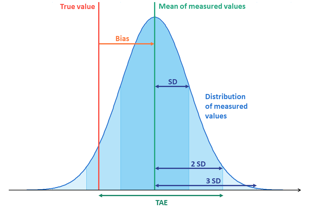
The idea behind TAE is pretty simple and intuitive, and it’s easiest to understand by looking at Image 3 that combines the previous two images of bias and variation.
In routine use, we, in most cases, only measure a sample once, so we cannot form this distribution for every sample individually to calculate the mean of measured values. But if we feel confident our verification describes the test’s behavior correctly in our patient samples, we can assume the bias and SD estimates found in the verification will describe the results in routine use too.
Now looking at Image 3 and remembering the previously introduced equations, we reach a certain level of confidence for our estimate of the total error related to a measurement by adding Z * SD to bias. Bias gives us the distance between the true value and the mean value, and Z * SD describes how much further from the true value the measured result can be with our selected confidence level. For example, with Z=2, over 95% of our results will stay within bias + 2 * SD from the true value. Correspondingly, it can be expressed as %bias + Z * %CV if it’s more appropriate to use proportional values.
Now let’s remind ourselves that bias can be either positive or negative. On the other hand, negative values for SD, %CV or TAE would not make sense since they only describe the expected error amount, not the error’s direction. Variation describes how much the result is likely to deviate from the mean value, and as we can see in Image 3, it’s just as likely to make the measured results smaller or larger than the mean value. Since variation can even make the measured result smaller than the true value in cases where bias is positive (and the other way round), we can neither make assumptions whether the measured result is smaller or larger than the true value. That’s why we don’t know whether the total error of a single measurement is positive or negative. Considering this, the equation for total analytical error becomes

where the small vertical lines denote that we are using the absolute value of bias.
Often this equation is presented as if bias was only the distance between mean and true value without the information about which is larger. If you are not interested in bias itself, it’s perfectly fine to omit the fact that it can be negative, and then you don’t need to state in this equation that we use the absolute value of bias. But in case your verification leads you to a conclusion that you need to calibrate your instrument, it’s important to know whether bias is positive or negative. That’s why we want to emphasize here the possibility of bias being negative.
When you calculate TAE with a quantitative accuracy study in Validation Manager, the default value for Z is 2 since a 95% confidence level is widely used in diagnostics. You can easily change Z to be something else if that suits your purposes better.
The recommendations for selecting Z vary. For example, with Z = 6, you can pretty safely say that none of the measured samples will have more error than TAE, as the probability of exceeding it would be somewhere around 1 / 1 000 000 000. But as Z = 3 is enough to give us information on the behavior of about 99% of all samples, in many cases, it’s not worth doubling the effect of random error in our TAE estimation just to get the tails of the distribution included. And in medical diagnostics, 95% confidence (Z = 2) is widely considered good enough. But that’s basically up to you, how you want to do this. For more information about TAE, we advise you to read materials by Westgard, e.g., Total Analytic Error: from Concept to Application (3).
The problem with TAE is that while it gives flexibility in how careful you want to be with your imprecision, the same does not apply to handling bias. If you set a performance goal for your TAE, the bigger your Z, the less sensitive your TAE is for changes in bias. This is problematic, because ideally, there should not be any bias, and therefore it is important to make sure that bias stays small. That’s why it is recommended to monitor bias separately if you only use TAE to estimate accuracy. In Validation Manager, you can do this simply by setting a goal for bias as well or by using another accuracy parameter side by side with TAE.
Measurement uncertainty
Measurement uncertainty describes the doubt related to a measurement. It combines error components from different types of error sources to form a single value to represent uncertainty with a selected level of confidence. The first international recommendation for measurement uncertainty was approved by International Committee for Weights and Measures (CIPM, Comité International des Poids et Mesures) in 1981.
In measurement uncertainty, the different components of uncertainty are combined as the sum of squares; similarly, as in ANOVA precision, we combine the different precision components to form within-lab precision: (%CVwl)^2 = (%CVwr)^2 + (%CVbr)^2 + (%CVbd)^2.
The purpose of calculating measurement uncertainty is to add all the different uncertainty components to the same equation to get an understanding of the overall uncertainty instead of just imprecision. Multiple factors cause uncertainty in the measurement, like humidity and temperature of the laboratory room, time of the day, or who runs the tests. To get them all included in your estimation for measurement uncertainty, you need to vary the conditions in your verification measurements so that all potentially relevant error components will have a chance to affect your results.
Since our options for measuring the effect of different uncertainty components is basically measuring imprecision and measuring bias, we can use these as the components of the equation:

Here k represents level of confidence. In Validation Manager, we use k = 2 because that corresponds to 95% confidence.
A geometrical representation of how U is calculated can be seen in Image 4. You can imagine looking at the result distribution from above. The circles represent the distribution of measured results similarly as in the image related to TAE. The mean of measured values is in the middle of the image. The smallest circle with the darkest shade of blue has a radius of 1 SD. The next circle around it has a radius of 2 SD, and the largest circle has a radius of 3 SD. The red dot on the left represents the true value. The green line that connects the true value and the edge of the circle with 1 SD radius is the result of the root of the sum of squares of bias and SD. With k = 2, we will need to double its length to get a value for U, and that is represented with a dotted line that ends somewhere between the edges of 2 SD and 3 SD circles. To make it easier to compare U with TAE, we’ve rotated the black line representing U horizontal. TAE would be bias + 2 SD (reaching horizontally from true value to the edge of 2 SD circle), so in this case, we can see that U is slightly larger than TAE.
The explanation above is a practical simplification of the concept of measurement uncertainty. The purpose of this approach is to be able to form an estimation for U based on measurements done within a limited time frame. Please note that there are often unexpected error sources that are not revealed during a verification. That’s why it’s good to find practices for monitoring U as part of your normal laboratory routines and to use the results of EQA to evaluate the reliability of your bias estimations.

A thorough description of the subject can be found in a GUM publication: Evaluation of measurement data – Guide to the expression of uncertainty in measurement (6).
How about RiliBÄK Delta
A somewhat similar parameter to U is RiliBÄK Delta, introduced by Rainer Macdonald in 2006 (8). Actually, it is not meant to be used for purposes of validation or estimation of measurement uncertainty but rather to be used as a quality control rule (9). It can nevertheless be calculated in Validation Manager alongside TAE and/or U.
What’s the difference and which to choose?
The difference between TAE and U is in the reasoning behind them: are we estimating error or uncertainty. If you are wondering how to set goals for these parameters, it might be good to know that in practice, with a confidence level of 95%, i.e., Z = 2 and k = 2, the values calculated for U and TAE are often not far from each other. If bias is less than double the SD, then the difference between the accuracy estimations given by U and TAE differ at most about 10% from each other. But if bias is bigger than 2 * SD, the difference between TAE and U grows fast, as U is more sensitive to bias than TAE.
For deciding which parameter to use, the first question is, what are you bound to do? ISO 17025 states that laboratories should estimate U. In Germany, RiliBÄK requires measuring Delta.
Additional relevant questions are:
- Do you need to compare your new results to your older verification results?
- Does your organization give you expectations on which parameter to use?
- Do you have peers with whom you compare your results so that you need to agree on what to measure?
- What kind of guidance do you have for setting the goals? For example, in clinical chemistry, it may be easier to find practical goals for TAE than for U.
If you feel you have conflicting needs, you can easily select all these parameters to be calculated from the same data set in Validation Manager. You don’t need to have goals for all of them, but setting some goals makes it easier for you to view your report and find the results that need more careful examination.
References
(1) J.O. Westgard, R.N. Carey, S. Wold (1974): “Criteria for judging precision and accuracy in method development and evaluation” Clin Chem. 1974 Jul;20(7):825-833
(2) J.O. Westgard, S.A. Westgard: “Total Analytic Error from Concept to Application” Clinical Laboratory News, Sep 1. 2013
(3) Extended version of previous article (Sep 2013) “Total Analytic Error: from Concept to Application“
(4) CLSI guideline EP29: “Expression of Measurement Uncertainty in Laboratory Medicine“
(5) CLSI guideline EP21 “Evaluation of Total Analytical Error for Quantitative Medical Laboratory Measurement Procedures“
(6) JCGM: “Evaluation of measurement data — Guide to the expression of uncertainty in measurement“
(7) Wikipedia: Measurement uncertainty
(8) R. MacDonald (July 2006): “Quality assessment of quantitative analytical results in laboratory medicine by root mean square of measurement deviation“ LaboratoriumsMedizin 30(3):111-117
(9) R. MacDonald (April 2007): “Reply to Haeckel and Wosniok: Root mean square of measurement deviation for quality assessment of quantitative analytical results in laboratory medicine compared to total error concepts“ LaboratoriumsMedizin 31(2):90-91
(10) Sten Westgard (July 2021): “New Goals for MU Goals“
(11) CLSI guideline EP10-A3: “Preliminary Evaluation of Quantitative Clinical Laboratory Measurement Procedures”
Accomplish more with less effort
See how Finbiosoft software services can transform the way your laboratory works.


